Results and discussion

Results

Test Case

Let’s consider the case of a forest in Kornanwand (Bas-Rhin, France) located at the West of Haguenau. This is a small forest amid fields.

The Location is define by it bounding box following the Well-Known Text (WKT) Standard (ISO/IEC 13249-3:2016). The coordinates are given in Lambert93 the standard Coordinate Reference System (CRS) in France.

On the map, the shape of the forest is represented as defined in BD TOPO.

Definition of the test case

Test Case: Kornanwand (67)
Description: Small forest surrounded by fields
Area:
Location: BOX(1036883 6868424, 1037070 6868616)
CRS: Lambert 93

Map 1. IGN Ortophoto map centered on Kornanwand

Starting Point

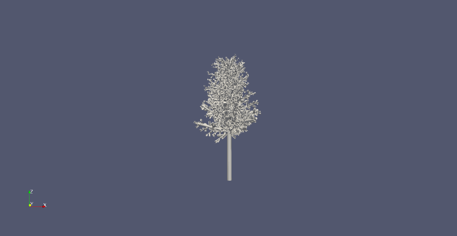
Figure 1. Structured Mesh of Kornanwand

Before my intership the forest were represented only by their canopy (figure 1). Using some of the algorithms describe above we will first detect the position of the tree using a local maximum filter then populatethe forest with trees generated by the method of Weber and Penn.

Detection

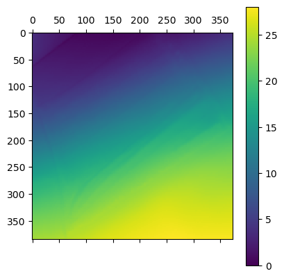
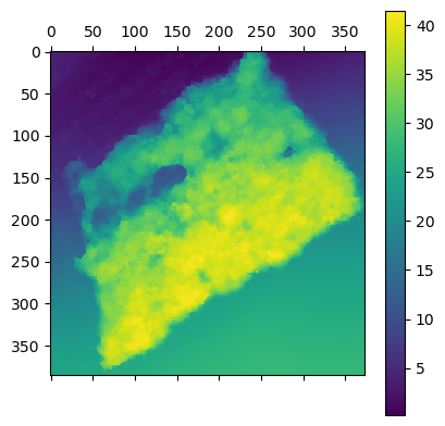
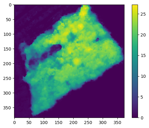
Th first Step in the detection of trees is to build a CHM. With the code I previously obtain I get the DTM and DSM the given zone. Then I computed the difference to get the height of the canopy (CHM)

Figure 2. DTM (colormap: size in meter)

Figure 3. DSM (colormap: size in meter)

Figure 4. CHM (colormap: size in meter)

To detect tree position I simply used a local maximum filter with the following parameters

min_distance: minimum number of space between to tree.
threshold_abs: minum size in meter to be classified as a tree.

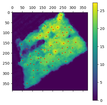
Figure 5. min_dist=10, threshold_abs=5

Figure 6. min_dist=5, threshold_abs=5

Figure 7. min_dist=10, threshold_abs=0

One can observe that the both parameter have a massive impact on the number false positive of false negative. In fact in min_distance is to high we miss trees and is threshold is to low we could classify ground point as trees.

Generation

Two trees generated with my implementation of the Weber and Penn model.

Figure 8. Quaking Aspen

Figure 9. Black Tupelo

Results

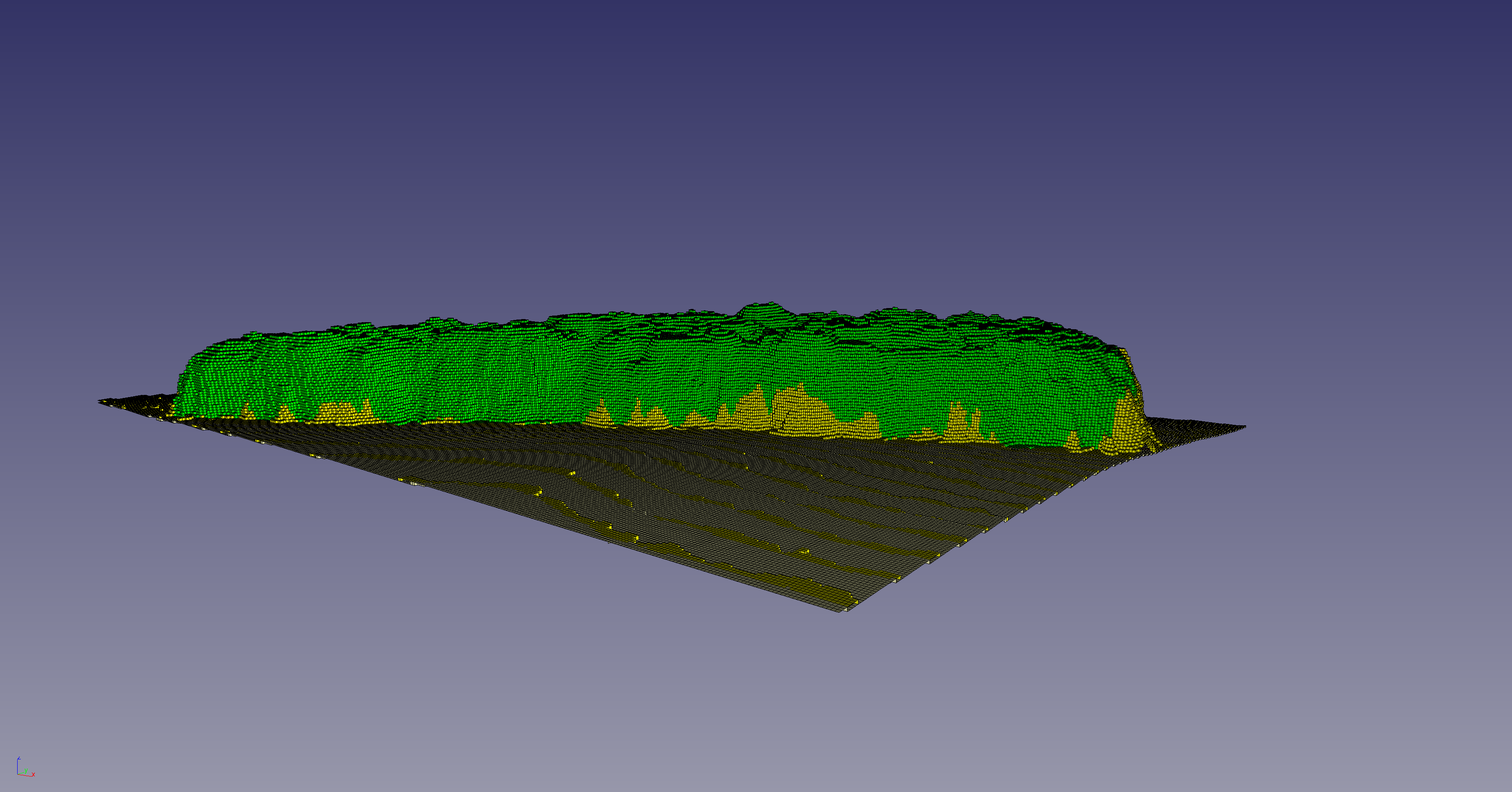
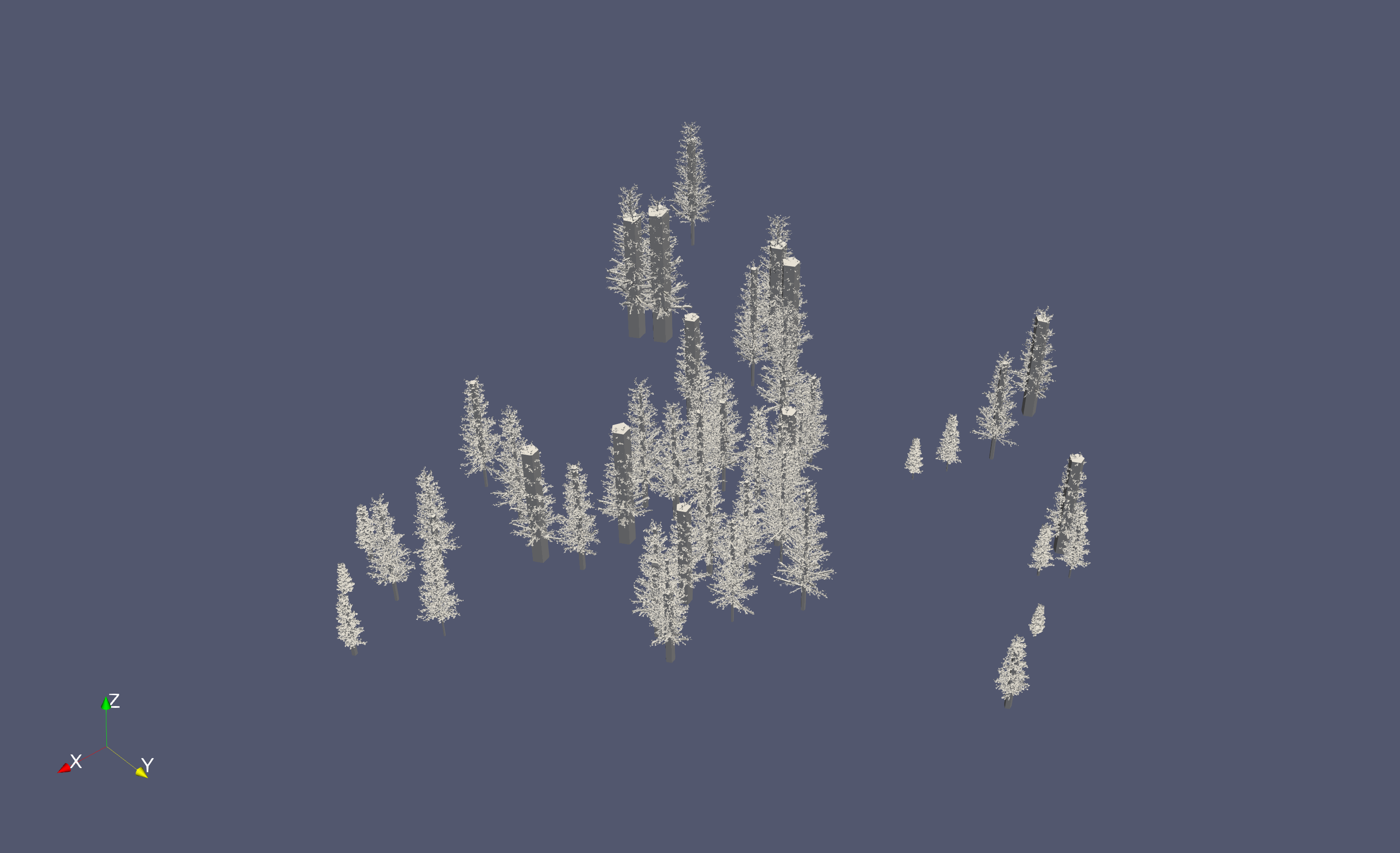
Combining the two results previously obtained I compute the discrete representation of the forest.

I ran the generation on a laptop with a quad-core CPU (Intel® Core™ i5-7300HQ CPU @ 2.50GHz) and 8 Gb of RAM.

The program was parallelized using the python multiprocessing library. It took 20 minutes to generate 150 trees. Each tree is generate on its own file in the .ply format.

In figure 1O, I displayed only a part of the forest, because my ram doesn’t allow me to display more.

Southern part of the forest

3d kw

Improvements

The tool I developed still requires some improvements.

Hybrid Method

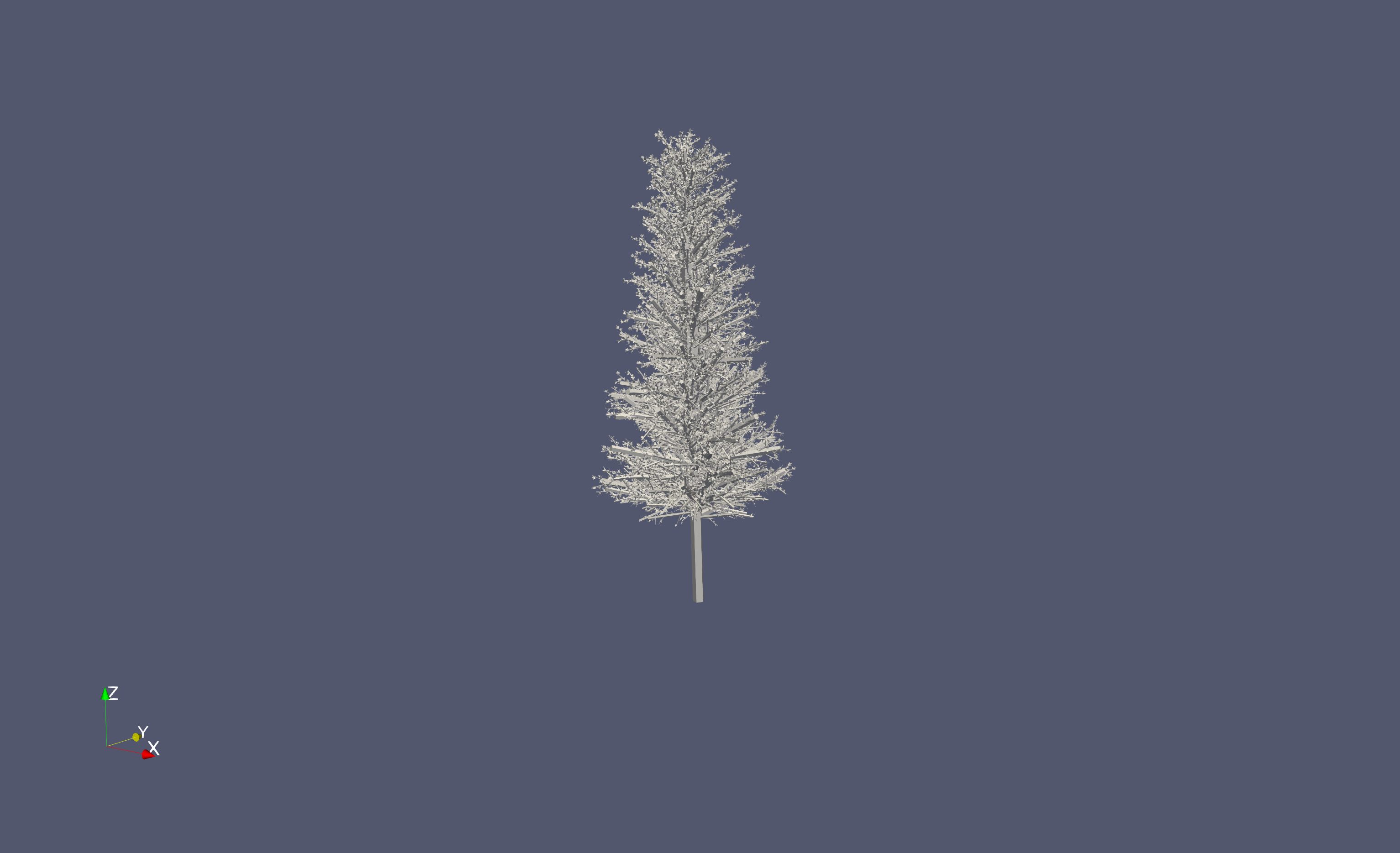
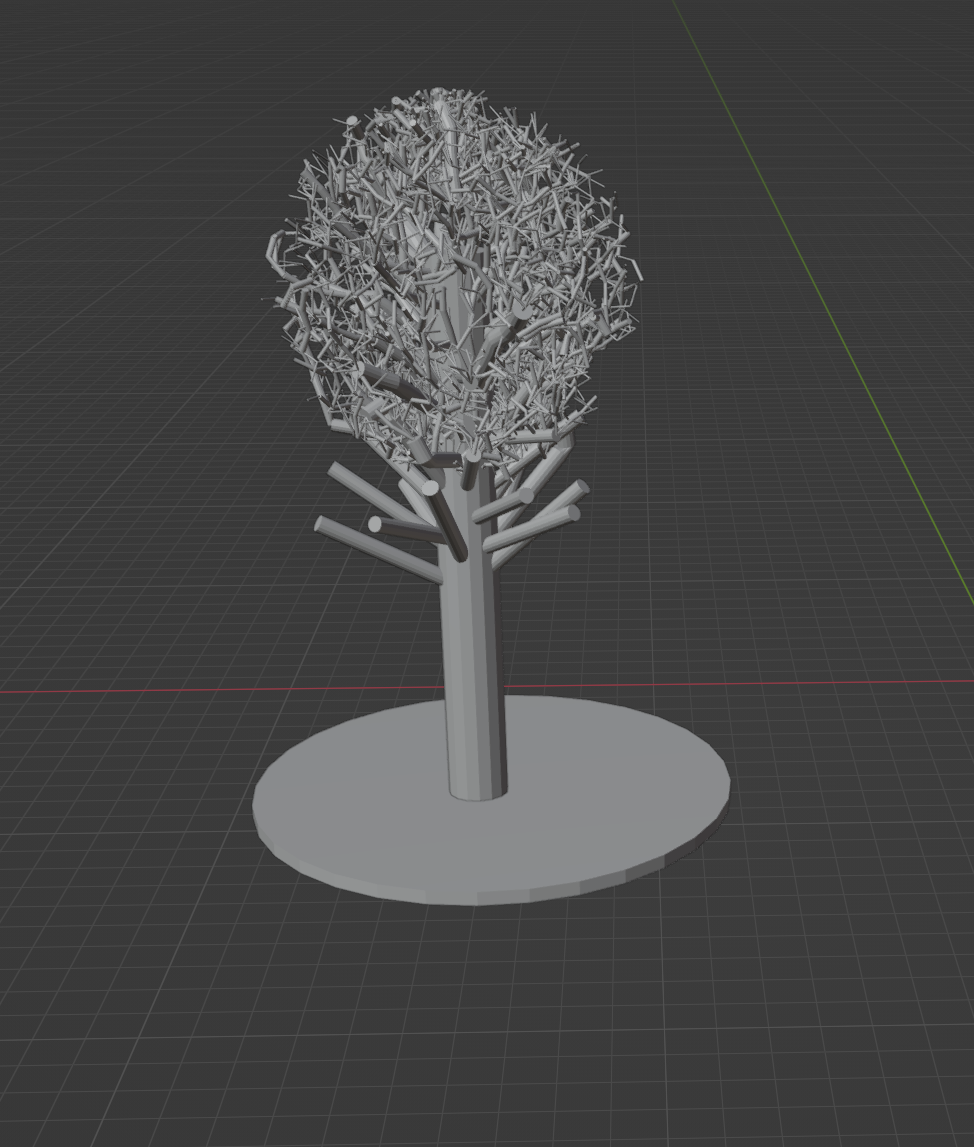
First the use of an hybrid method between using Weber and Penn to initialize the space colonization algorithm would be a good compromise to speed up and fit more closely to the DSM. Though this hybrid is in development (figure 11).

Figure 10. Weber and Penn + Space colonization

Detection

To be applying the space colonization algorithm needs to be feed attraction point, to do so segmentation algorithm like Dalponte or Silva should be applied.

Performance

The implementation was made using python, this could be speed up by integating some C++ and by using MPI for the parallelization. Each beeing contruct independantly from it’s neighbourgs, it will be easy to integrate MPI to the code as it would require few communication between the threads.